Table of Contents
OVERVIEW
This chapter presents a conceptual overview for the production of computer graphics for instruction. The goal is not to teach the use of any one particular graphics application, but rather to provide an organizer for the different approaches commonly found on microcomputer systems and to give a sense of what features and effects currently exist. The development of static and animated computer graphics are considered separately. The chapter also introduces the concept of "second-hand" graphics, including those produced from scanning print-based pictures or capturing video snapshots and then converting the images into digital form for later use on the computer.
OBJECTIVES
Comprehension
After reading this chapter, you should be able to:
Application
After reading this chapter, you should be able to:
This chapter deals with issues surrounding the development of computer graphics for instruction. The differences and relationships between design and development are analogous to those between the blueprint and construction of a house (Reigeluth, 1983b). Design proposes instruction and describes its specifications, often in great levels of detail. Development concerns the actual production or "construction" of the design. Changes to the design are easy and relatively inexpensive. Changes to the development can be costly and time-consuming. This is not to suggest that design and development are mutually exclusive. In fact, some media, like computers, often permit an instructional materials production cycle where design and development are intertwined. This approach, called rapid prototyping, is discussed in more detail in chapter 7. At the very least, designers must consider the resources, conditions, and constraints of development.
Instructional designers, like their counterparts in architecture, must consider many tradeoffs and compromises throughout the design and development phases. Instructional designers must carefully consider how decisions affect groups of instructional variables, just as the decision to use two-by-four-inch lumber, two-by-six-inch lumber, or fabricated metal incurs tradeoffs among cost, strength, and installation time.
Instructional designers and developers often talk about the relationship between instructional effectiveness and efficiency. No instructional design can ever hope to be perfect in every respect. Consider the situation of learners achieving 85%, instead of 95%, of the "goals" of the instruction. A designer must ask whether it is worth the time and cost to revise the instruction to attain the extra 10%. Obviously, the answer is based on the context and will be different, for example, for the training of medical personnel on emergency room procedures versus elementary instruction on art appreciation. Of course, saving time and money is meaningless if the instruction, like the house, falls apart after it is built. This is a little like buying a pair of pants that are the wrong size just because they are on sale. The hope is to maximize effectiveness while minimizing cost, design time, development time, and instructional time (i.e., the time required by a learner to complete the instruction).
The purpose of this chapter is not to provide instruction on the "how to's" of computer graphics applications. Teaching how to use even a small number of specific commercial graphics applications is not a goal of this book. The rapid rate at which new commercial graphic software packages are introduced, combined with the fickle nature of developers and users, would make this chapter obsolete before the ink dried. Instead, the goal of this chapter is to provide a brief conceptual overview of past, present, and (hopefully) future approaches to developing computer graphics. It is important to note that this chapter will focus entirely on graphics produced from microcomputer systems.
Since this is a book concerned with the design of computer graphics for instruction, one might question why development is even considered at all. There are several reasons. As already mentioned, design and development are not independent of one another. Knowledge and sensitivity about development issues influence design decisions. For example, although design may call for an animated sequence, knowledge about the capability and cost (in terms of money and time) of the particular microcomputer system will influence how elaborate the sequence can be, as well as the possibility of changing the design altogether, such as to a sequence of multiple static graphics. A final reason to consider development is simply to gain some sensitivity and appreciation for the rapid advancement in graphics production on microcomputers.
HARDWARE SYSTEMS: TYPES OF COMPUTER GRAPHICS DISPLAYS
Regardless of how a graphic is produced on a computer, the end result will be either a computer display of the graphic or a computer file that stores information about the graphic, or both (Artwick, 1985). There are three fundamental structures, known as graphic primitives, that act as the building blocks for all computer graphics (Pokorny & Gerald, 1989). The first is the picture element, or pixel, which is simply a single point of light on the computer screen. The next two elements are the line and the polygon. All computer-generated images can be created from these three graphic primitives.
Essentially there are two major kinds of computer graphics display systems that can produce pixels, lines, and polygons: raster graphics displays and vector graphics displays (Conrac Corporation, 1985). Each uses a fundamentally different hardware approach to controlling the scan rate and pattern of the cathode-ray tube (CRT) to display the graphic. Vector graphics displays, as the name implies, use vectors to define lines, which, in turn, comprise polygons. A vector is a mathematical entity comprised of two or more elements. A line, for example, is defined on a vector display in terms of its magnitude (e.g., length) and direction. Diagonal lines on vector graphics displays are true diagonals and do not suffer from the "jaggies" associated with the more common raster graphics displays. However, virtually all desktop computer systems use raster graphic displays.
Raster graphics are formed by a pattern of pixels on the computer screen. A single graphic consists of a matrix of on or off pixels (or "0" or "1," either of which defines a "bit" of information on a computer). For this reason, raster graphics are sometimes referred to as bit-mapped displays. One can more easily understand bit-mapped graphics by imagining that the computer screen is a matrix of tiny light bulbs. In order to draw the letter "H," the computer must be told which light bulbs (pixels) should be off or on, such as shown in Figure 3.1. Information related to shades of gray or color could also be stored in relation to each pixel.
In general, displaying a black and white bit-mapped graphic consumes the same amount of computer memory, regardless of the simplicity or complexity of the graphic display, because it takes the same amount of memory to store information about each pixel whether it is off or on. (See Footnote 1) Scanning and digitizing processes transform analog images, such as line drawings and photographs, into the digital form of bit-mapped graphics. An everyday example of graphics produced by the combination of dots, apart from computers, are photographs in newspapers. The continuous tones of shading in a photograph must be broken down into tiny dots of varying size and intensity. The resulting image, called a halftone, is printed in the newspaper as a reproduction of this configuration of dots. From a distance, the human eye perceives continuous shades of gray from the discrete collection of dots.
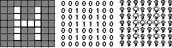
Figure 3.1
Raster graphics are formed by a pattern of "pixels" on the computer screen. A "bit" map of a graphic, such as the letter "H," is analogous to a pattern of lit light bulbs, where "1" means the light bulb is on and "0" means the light bulb is off.
The clarity and sharpness of a bit-mapped graphic, known as resolution, depends on the number of pixels contained in a certain display area. Low-resolution displays offer crude graphic representations because the smallest point of light that can be manipulated is quite large. Increasing the resolution means increasing the number of rows and columns in the graphic matrix to produce a greater number of smaller and smaller pixels in a given area, such as that shown in Figure 3.2. High resolution is a function of the level of detail produced by the pixel size and is therefore relative to the capability of the computer hardware.
A diagonal line presents problems on raster displays because of the row and column orientation of the pixels. Diagonals often have a jagged look resembling a staircase, such as the exaggerated example in Figure 3.3. This effect is minimized as the resolution of the display is increased. A high-end software technique, called antialiasing, also can be used to minimize the jagged effect by averaging the shading of pixels adjacent to the diagonal.
PRODUCING STATIC COMPUTER GRAPHICS
This section presents a brief conceptual overview of the software approaches to produce computer graphics on microcomputer systems and how these graphics can be electronically stored for future use.
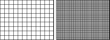
Figure 3.2
A comparison of low-resolution (left) and high-resolution (right) display screens.
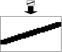
Figure 3.3
Diagonals displayed on raster systems are prone to the "jaggies." In this example, a diagonal is enlarged many times to show the way individual pixels are "staircased." The greater the screen resolution, the less the distortion.
One can produce computer graphics on microcomputer systems in essentially one of three ways:
The command-based approach involves algorithmic processes for defining a graphic, such as the writing of programming code using special graphics commands particular to the programming language (e.g., PASCAL, C, BASIC, LOGO).
The GUI-based approach is based on the graphical user interface discussed in chapter 1 and involves graphic tools such as "pencils," "brushes," "fill buckets," "box makers," etc. GUI-based approaches most commonly use input devices such as a mouse, light pens, and graphic tablets, although some of the earliest GUI-based approaches used the keyboard. The GUI-based approach is now the status quo on most microcomputer systems. Some authoring environments, both old (e.g., PILOT) and new (e.g., HyperCard, Authorware), offer a combination of command-based and GUI-based approaches.
Second-hand graphics are copied, not created, and include clip art and all of the scanning and digitizing technology (both hardware and software). For example, graphics can be drawn on paper, converted into digital form with a scanner, and then "imported" into one of many computer applications. This approach also includes the electronic "capture" of video and photographic images.
Each of these three approaches will be briefly described, after an overview of various formats in which graphics can be stored on disk.
Overview of Graphic File Formats
Command-based, GUI-based, and scanned/digitized graphics can be stored in a variety of formats on a computer disk (floppy, hard, optical, or compact), as listed in Table 3.1. The format of a stored graphic image directly affects the way it can be used or revised later. For example, when computer graphics are stored as bit-mapped images, only the "on/off" pixel pattern is saved. Bit-mapped files are commonly known in some systems as paint files. TIFF (Tagged Image File Format) files also store bit-map graphics, but can include additional grayscale and color information.
Other formats allow a graphic to be stored on disk as a collection of one or more individually defined and editable "objects." (See Footnote 2) These files are sometimes referred to as drawings. Instead of storing the actual graphic as a bit map, the visual attributes of the graphic are stored as a group of mathematically defined objects. In this way, the graphic is simply redrawn by the computer every time it is retrieved from disk to random-access memory (RAM). Almost all of the latest graphics packages that use the GUI-based approach store the graphic in this way. Most graphics packages save the drawing in a format that is specific to the software. In addition, some graphical programs allow object-oriented drawings to be converted to bit-mapped paint files. Once converted to a bit map, individual information for each of the drawing's objects is lost.
|
|
Paint file -- graphic stored as bitmap Drawing -- graphic stored as a group of one or more editable objects Pict file -- generic graphic file format for both bitmap and object-oriented graphics
|
Several generic formats have been created to allow a graphic to be stored and imported into a wide range of applications. One common format, called a pict (for picture) file, can store both bit-mapped graphics or object-oriented drawings. Most major brand-name graphics software packages can both read and save pict files, allowing for easy swapping of graphics from one application to another. Many word processors, desktop publishing and presentation packages, and authoring packages are only able to import pict files.
There are a variety of specific file formats available, depending on what hardware and software are used. Readers can take both warning and solace in knowing that the issue of multiple-storage formats often confuses and bewilders novice computer users, even though it is not really that complicated. In order for a graphic to be used in an application different than the one in which it was created is analogous to home plumbing problems, such as trying to connect 1/2-inch and 5/8-inch pipes. In order to get a graphic from "here to there," some kind of "adapter" must be used as an in-between step, such as first converting one specific drawing format to a pict file before importing it into another application. This is a good example of an idea more easily understood by actually working with a computer than reading about it in a book.
Computer graphics also may be stored as a computer program. This is not considered a graphic file format because the graphic itself is not stored, only the idea of the graphic as represented in the all verbal form of the computer program. Most common programming languages on microcomputers have graphic commands and functions. The next section elaborates on this idea.
Command-Based Approaches to Producing Static Computer Graphics
Long gone are the days when computer company executives argued about whether to include upper- and lowercase letters on their computer terminal displays. When microcomputers became readily available in the late 1970s and early 1980s, the main way to produce graphics was to master one of several programming environments. True hackers learned low-level programming languages, such as assembler and machine code. However, the opportunity to access low- and high-resolution graphics "pages" through graphic commands in high-level programming languages, such as BASIC, LOGO, and PASCAL, made graphics a popular and easy (relative to machine code) context for programming projects. Command-based approaches are typically based on a Cartesian coordinate system. However, another creative, though less well-known system, called turtle geometry, also has been used.
Cartesian Coordinate System
Anyone who has played "Bingo" or "Battleship" is already well acquainted with the idea of dividing a flat space into a grid system in such a way as to precisely define a specific location on a two-dimensional surface. A system based on Cartesian coordinates (named after French mathematician René Descartes) is simply a formal mathematical approach for doing the same thing. Figure 3.4 shows a typical example of such a system, which would be recognized by any first-year high school algebra student. In a two-dimensional plane, a set of Cartesian coordinates consists of two numbers, each separated by a comma. The first number refers to the horizontal (or X) axis, and the second number refers to the vertical (or Y) axis. A traditional Cartesian system is separated into four polar (i.e., positive or negative) quadrants, depending on values of each of the coordinates. Most computers usually only use the positive/positive quadrant, although it is often modified such that it is "flipped," making the point of origin (0,0) reside in the top left corner of the screen, as illustrated in Figure 3.5. Users simply need to remember that the screen is divided into a matrix of rows and columns starting with point 0,0 and extending as far as the resolution of the particular system permits (e.g., 512, 342 in the case of the standard Macintosh screen).
Drawing screen graphics is really just a matter of playing "connect the dots" through a variety of graphical programming commands. Although programming languages vary in their names of specific commands, the fundamental functions of these commands are very similar across languages. In order to draw a box, for example, one must draw a series of four lines from, say, point 50,50 to 100,50 to 100,100 to 50,100, and back again to 50,50. (Figure 3.6 shows two small programs that accomplish this task.) Of course, some programming languages will have more commands covering a wider range of graphic functions than others. For example, many languages have special commands that allow simple objects, such as boxes and ovals, to be drawn more quickly by defining the objects in terms of its diagonal, as shown in Figure 3.7.
The graphic could be saved either as the program consisting of the series of graphic commands or as a bit-mapped image. If saved as a program, the visual representation of the graphic itself is not stored, only the algorithm, which, when run, produces the graphic. In terms of computer memory, the size of the stored file depends directly on the length of the program, not on the complexity of the graphic image. Our box example would only require the storage of a few simple lines. Saving it as a bit-mapped image, on the other hand, saves only the visual representation currently appearing on the computer screen. This bit-mapped image can be recalled later, but the computer has no way of knowing how it was created. The computer merely retrieves and reconstructs the matrix of on/off pixels. The memory to store a graphic as a bit-mapped image is the same whether the graphic was actually produced by one line or 1,000 lines of programming code.
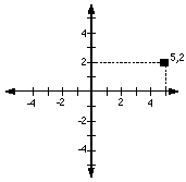
Figure 3.4
An example of a Cartesian coordinate system.
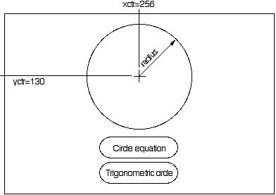
A more interesting example of "connect the dots" strategies concerns graphics that contain curves, such as circles, ellipses, and arcs. As already mentioned, many languages include "oval makers" to produce the oval represented within the perimeter of an imaginary rectangle. Lacking such a functional tool, we are left with the task of defining our own circle as a collection of connected dots. Since a circle is mathematically defined as an infinite number of points equidistant from its center, compromising is essential. Rather than draw a true circle, a polygon can be constructed to represent a circle -- the more sides, the better the representation. We can either manually decide which pixels will be connected or we can use a mathematical model of a circle and let the computer compute the dots. Box 3.1 demonstrates two examples of the latter approach, using modifications of the traditional formula for defining a circle with Cartesian coordinates and another based on trigonometric functions. This is a simple example of using a pure mathematical model for driving the production of computer graphics and is essentially the same concept used in the most sophisticated computer-assisted design (CAD) systems.
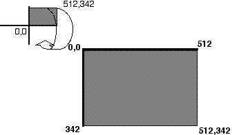
Figure 3.5
The coordinate system as used on the standard Apple Macintosh screen. This system is based on vertically "flipping" the traditional positive quadrant.
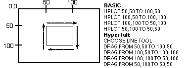
Figure 3.6
Two programs that draw a box by connecting lines from each of the box's corners.
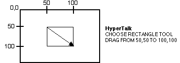
Figure 3.7
A program that draws a box as defined by its diagonal.
Turtle Graphics
Although command-based approaches to producing computer graphics are usually based on the Cartesian coordinate system, there is one other notable and unique way to do it. This approach, called turtle graphics, was initially developed for use with the LOGO programming language and was founded on learning principles associated with the process of creating the graphic, and not on the product itself (i.e., the resulting graphic image) (Abelson & diSessa, 1981; Lockard, Abrams, & Many, 1990; Papert, 1980). (See Footnote 3) In other words, the goal was to find a way for people of varying ages and ability to think and communicate about geometry without using the rather cryptic (and often meaningless) method associated with Cartesian systems. The LOGO language capitalized on the use of graphics to allow users, even young children, to gain access to powerful ideas associated with mathematics and computers. LOGO is often misinterpreted as a "toy" language, but in reality it is a sophisticated procedural programming language. Turtle graphics is but one of many "microworlds" users can explore in LOGO.
As the name implies, users create graphics by manipulating a graphic object, called a turtle, on the computer screen. As users "drive" the turtle, it leaves a trail. The turtle has vector-like qualities in that it has two characteristics -- position and heading. Turtle graphics is a fundamentally different approach to mathematics when compared to the more common and traditional approach based on Cartesian coordinate systems. Cartesian systems define a figure, such as a circle, by its relative position to a set of points outside of the figure, such as a perpendicular axes, and an Euclidean system defines it in relation to one inside point, its center. Turtle graphics, on the other hand, defines the figure in relation to the relative position of the turtle on the figure itself. For this reason, turtle geometry is based on differential or "intrinsic" mathematics. Whereas Cartesian systems define graphics on the basis of fixed, absolute points, turtle graphics are drawn by commands that are relative to each other. The movement of one turtle graphic command is always in relation to its position and heading immediately before the command's execution. For example, the command FORWARD 50 will draw a line in whatever direction the turtle is pointing.
Some of the most common turtle graphic commands, called primitives, are shown in Figure 3.8. In order to draw a box, for example, a series of FORWARD and RIGHT commands must be executed, as shown in Figure 3.9. Some very interesting and powerful mathematical ideas can be expressed and explored with just this small list of commands. To draw a circle, the idea of "move a little, turn a little" is repeated until the turtle has made a complete "round trip" and arrives back at its original position with its original heading, also shown in Figure 3.9.
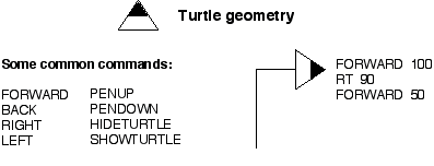
Figure 3.8
Some common commands of turtle geometry.
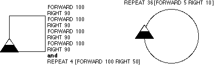
Figure 3.9
Two sample turtle geometry programs that draw a square and one that draws a circle.
|
|
|
Here are two examples in which circles are drawn mathematically. The first example is based on the traditional circle formula: where h,k are the coordinates of the center of the circle, r is the radius, and x,y are the coordinates of any one position on the circle itself (and ^2 means to square this quantity). The second way defines the x,y position on the circle using the trigonometric functions of sine and cosine. Both examples are presented using HyperTalk, the language of HyperCard on the Apple Macintosh (also known as scripting). The scripting on the following page corresponds to each of the two "buttons" shown on the "card" below:
One positive consequence of this approach, assuming you are successful, is that you will really understand what the mathematics of the formulas mean. Chapter 8 will discuss this issue of empowering students with tools, such as the computer, to help them understand the process of mathematics and science. Here is a legend for the major variables in each of the two scripts that follow: xctr -- horizontal coordinate of the center of the circle yctr -- vertical coordinate of the center of the circle rad -- the radius of the circle x -- horizontal coordinate of any one position on the circle y -- vertical coordinate of any one position on the circle Script of card button "circle equation:"
|
GUI-Based Approaches to Producing Static Computer Graphics
Programming a sequence of commands, even in turtle geometry, is a very abstract way to draw a picture. A much more concrete method, based on the idea of the graphical user interface (GUI), comes closer to the everyday experience of actually sketching a picture with paper and pencil. GUI graphics applications have a variety of graphics tools, functions, and effects. Selecting these tools, functions, and effects, and then using them to draw a graphic is done with one of any number of input devices. GUI-based approaches work fundamentally the same way, irrespective of which input device is used. The most direct approach is using a light pen to actually draw on the computer screen. Pressure-sensitive graphic tablets or sketchpads also can be used. The user draws on the tablet with a blunt stylus. The motion of the stylus on the tablet is mirrored on the computer screen. The feel of these electronic sketchpads is less natural than light pens, and it usually takes awhile to develop the necessary eye-hand coordination. In between the light pen and graphics tablets on the "feel scale" is the mouse -- a hand-held device with one or more buttons that mirror the motion of the user's hand. Mouse users have their own vocabulary as they point to and manipulate screen objects, such as "aim and click," "double-click," and "click, hold, and drag."
Two main types of GUI-based graphics packages are available, painting packages and drawing packages, which are named closely after the way the graphics are stored. Paint packages are analogous to painting or printing directly on a sheet of paper with a pencil or pen. (See Footnote 4) After the graphic has been painted, it cannot be edited or modified. Instead, you have to use an "eraser" to correct mistakes and make changes or "cut" out entire sections of the graphic. As one might guess, graphics produced by painting packages can only be saved as a bit map.
Drawing packages, on the other hand, allow a graphic to be composed of one or more objects, each of which can be continually edited and modified. Figure 3.10 shows a screen snapshot of a graphic package called MacDraw II for the Macintosh. The features found in MacDraw II are typical of drawing packages. The menu bar across the top of the screen designates categories of graphic and text effects, as well as file functions such as saving and printing. Just below the menu bar and title line are some of the many patterns that can be used to "fill" any screen object created (including simple objects like straight lines). A palette of graphic tools is shown on the left edge of the screen. Horizontal and vertical rulers mark the dimensions of the drawing page. The slide bars on the right and bottom edges of the screen let the user move the drawing page around the screen (necessary because the computer screen can only show a small portion of the entire drawing page at any one time; most packages use 8 1/2-by-11-inch paper as the standard size, but this can be greatly expanded).
The screen arrow, controlled by the user via the input device (like the mouse), is used to select any tool, function, or effect, as well as for drawing. It is common for the screen arrow to change shapes to reflect its particular function at any time. For example, as an arrow, it represents a selection tool. When freehand drawing, it may look like a pencil or a paint brush. As this example shows, a GUI-based approach uses many graphical symbols to represent the tools and functions, such as the box tool, oval tool, and line tool. Some of the other symbols are less obvious. The capital letter "A" represents a text editor to generate and modify text objects. The pair of "mountains" at the extreme bottom-left edge of the screen either enlarge or reduce the view of the drawing page.
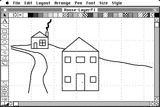
Figure 3.10
An example of a typical graphics package based on a graphical user interface (GUI).
Just as an artist working with traditional drawing materials, a computer graphic is produced in a GUI-based approach by alternately selecting and using tools, functions, effects, and other features (such as color). Most GUI packages are object-oriented, meaning that as objects are drawn they retain their separate identities. This allows them to be moved, edited, and copied. Hence, any one drawing is comprised of a collection of individual objects.
Examples of Typical Functions and Effects
There are too many graphic tools, functions, and effects across the many applications currently available on the market to possibly describe them all. However, the next section describes a core set of functions and effects common to many graphics packages.
Grouping and Ungrouping Objects. Even a simple graphic like a house is made up of multiple individual objects. The walls, door, window, roof, chimney, smoke, roadway, and pasture in Figure 3.10 are all separate objects. It is therefore much more convenient to group the separate objects into meaningful sets, such as all of the objects that comprise each house (e.g., door, window, roof, etc.). The grouped object then can be manipulated in the same way as any other object. When needed, the house can be ungrouped at any time.
Object Arrangement. When objects overlap, it is often necessary to define which object should be "on top" or "in front of" the other. This is analogous to cutting out figures from construction paper and laying them down on top of each other. Most GUI systems allow any object to be moved progressively "backward" or "forward." The arrangement of objects is particularly important when each closed object has been filled with a pattern or color. When no pattern or color has been chosen, the objects appear transparent, or as simple line drawings.
Alignment. Freehand drawing on a computer is a tough task. It is extremely difficult to precisely control most input devices, like the mouse, no matter how steady your hand. In order to provide greater accuracy in drawing objects, most packages allow objects to "snap" to imaginary grid lines in small increments, such as one-eighth-inch increments. This feature is similar to the kinds of control and accuracy necessary in computer-aided design. This feature usually can be turned on and off at will.
Rotation. Once an object is created, its orientation on the screen usually can be changed. Almost all systems allow an object to be "flipped" vertically or horizontally, but rotation features are particularly useful. Most packages allow an object to be rotated freely, as well as constraining the rotation to increments of 15, 30, 45, or 90 degrees. An example of rotating an object is shown in Figure 3.11.
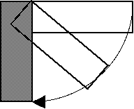
Figure 3.11
An example of rotating an object 90 degrees.
Layering. Complicated graphics can consist of hundreds of objects. Many packages allow a complex graphic to be constructed in layers, such that once a layer is defined, it becomes part of the background. The user cannot manipulate objects except those on the currently active layer. This helps the user organize the graphic and helps prevent accidentally selecting the wrong object. Layering is analogous to constructing one graphic on several plates of glass, each stacked on top of one another, as shown in Figure 3.12. Any one "plate," or layer, can be drawn on at a time. Once drawn, the layers can be stacked in any order. Just like grouping, the objects on layers above will cover objects on layers below. The simplest example would be a graphic consisting of two layers, where the one below acts as the background.
Line Smoothing. Freehand drawing of smooth, rolling curves on a computer is very difficult. When using paper and pencil, one can use a variety of sketching techniques and tools, like plastic templates, to make the task easier and to improve quality. These techniques just do not work well on a computer. Many packages, however, allow irregular curves to be constructed as a series of straight lines comprised of "valleys" and "peaks," which are then "smoothed" over by the computer, as shown in Figure 3.13. The low and high spots of the curve become "handles" with which to modify the curve.
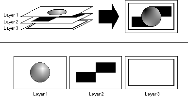
Figure 3.12
The concept of layering. In this case, one graphic is comprised of three separate layers, each of which can be edited. The layers can be rearranged in any order. Any one layer can be deleted and more layers can be added, if necessary.
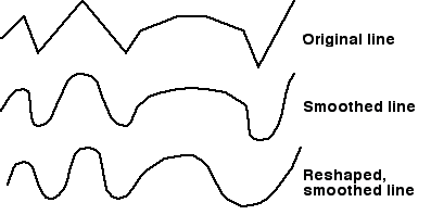
Figure 3.13
The concept of line smoothing.
Graphing. The capability to create spatial representations of categorical and numerical information, such as line graphs, bar graphs, and pie graphs, represents a distinct set of graphics applications. These and other graphing functions are usually provided in separate graphing software packages that construct graphs based on raw data entered by the user, such as that shown in Figure 3.14. However, graphing functions are becoming a more popular feature of many commercial spreadsheets.
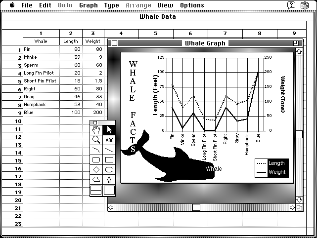
Figure 3.14
An example of a graphing package. The user enters raw data and the software subsequently constructs one of many possible graphs.
Second-Hand Computer Graphics: Clip Art, Scanning, and Digitizing
Despite the many features and effects that graphics applications now provide and the many more they likely will provide in the future, there always will exist two inherent user limitations related to creating an original computer graphic -- talent and time. Professionals increasingly turn to two alternative methods to get high-quality computer graphics in their materials. Neither method demands much talent because, instead of creating an original graphic from scratch, you either find and borrow a graphic drawn by someone else or take a photograph and convert the picture to digital form. We will refer to these as "second-hand" graphics to distinguish them from the graphics a user draws from scratch.
The most popular form of second-hand graphics are called clip art files. The idea is simple: Hire computer graphics artists to draw a collection of graphics using common graphics applications. The files can be sold to users who can load, use, and edit the files as if they had drawn the graphics themselves, as shown in Figure 3.15. The idea of clip art is not new; it has been used for many years in the printing industry. Most arts and craft stores sell print-based clip art that can be cut with scissors and used in newsletters and other publications. Although many companies produce and sell clip art, computer user groups frequently swap graphics files among members. Commercially produced clip art is usually sold with the understanding that the user is given the right to reproduce the art work freely in whatever work it is needed. Unfortunately, copyrighted graphics are also frequently shared in this manner among users; reproducing copyrighted material without permission is, of course, illegal.
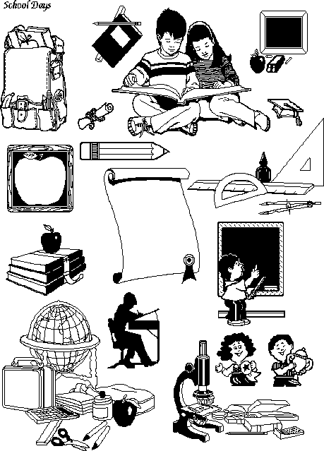
Figure 3.15
An example of "clip art."
Second-hand graphics also can be created by converting analog images, such as print-based or video pictures, to digital form. Optical scanners are probably the most common device used for this purpose. A typical hardware configuration is shown in Figure 3.16. Optical scanners work in much the same way as paper copiers. The document to be scanned, typically called the original, is usually placed face down on a glass plate. A bright light is pulled across underneath the original to detect variations in the amount of light reflected back, called reflective density.
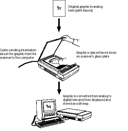
Figure 3.16
A computer interfaced with an optical scanner.
Scanners vary in the amount of information that is sent back to the computer for each point scanned in the original, and this information is used to define one of several composition types. The simplest, known as line art, is when each scanned point is recorded as either black or white. Most scanners allow for the handling of shades of gray. Some use halftone patterns, similar to that used in a newspaper photo. Others use grayscale settings, where continuous shades of gray are approximated. Finally, the most sophisticated scanners can record color.
Various software features allow the user to change various scanning settings. The threshold setting determines whether a specific dot on the original is recorded as black or white. Other common settings include the ability to change the brightness, or the degree of overall whiteness of the image, and the contrast, or the relative difference between black and white. At the highest contrast settings, black and white are emphasized and few gray shades are left. At the lowest contrast settings, the scanner emphasizes the middle gray shades, leaving little which is pure white or black.
Obviously the more information a scanner records about an image, the more computer memory is needed to store the file. Fairly simple graphics about the size of a typical computer screen can take as little as 5 to 10 kilobytes for simple line art drawings. Grayscale images, on the other hand, must record an exact shade of gray for each scanned dot. For example, a scanner that records one of 16 shades of gray for each dot must use four bits of memory for every scanned point in the original. At the extreme end, it is not uncommon for a scanned color image to contain up to one megabyte (approximately 1 million bytes) of memory. Regardless of the brand and the features, the issues of economy and processing ability related to computer memory become very important to understand.
There are other examples of devices that allow images or objects to be digitized, including specially designed or adapted photographic or video equipment that takes digital snapshots of real objects. Scanning and digitizing technology is advancing at a tremendous rate and is worth watching over the coming years.
PRODUCING ANIMATED COMPUTER GRAPHICS
Similar to static graphics, animated graphics can be produced either by a command-based or GUI-based approach. Producing animated displays with command-based approaches are really just extensions of the techniques discussed in relation to static graphics. On the other hand, GUI-based approaches can vary greatly from one animation package to another. We will discuss various approaches, starting with some simple, yet fundamental ideas, and then proceed to other, more sophisticated, approaches. It is useful to understand development issues of animated displays in terms of two animation designs: fixed-path and data-driven.
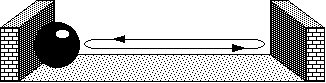
Fixed-path animation is analogous to choreographing a movie sequence. The same exact animation is supposed to happen the same way, in the same place, at the same time, each and every time the sequence is executed. Fixed-path animation, therefore, is a good technique when a design calls for a specific presentation of an animated sequence. We will consider some of the fundamental programming techniques in creating computer animation. However, many GUI animation packages offer the ability to record the real-time motion of a screen object while a user simply moves it around the screen. The software can then play back the animation just as it was "performed." The software does all the dirty work for the developer, such as storing and processing all of the mathematical operations actually responsible for the animation to take place.
In contrast, motion and direction of screen objects in data-driven animation do not vary according to the actual movement of the human hand, but by some data source. Although fixed-path animation also can be created by a data source and then "captured" or "recorded,"(See Footnote 5) we will define the data in data-driven animation as that generated by the student during the instructional sequence. Visually based simulations, such as flight simulators and video games, are good examples of what we will call data-driven animation. By our definition, animation is produced in real-time, or in the actual time that the user watches the display. In this way, the animation acts as visual feedback to students as they interact with the simulation moment to moment. Obviously, there is no way to anticipate when or if a particular student will "dive" or "climb." Instead, a mathematical model of the physical environment being simulated must be programmed into the computer in such a way as to refresh the graphics realistically in order to create the illusion that the student is actually controlling the "plane." Whereas fixed-path animation does only one thing, data-driven animation, theoretically, can produce an infinite number of displays with a finite amount of information. Both fixed-path and data-driven animation can be manipulated in one, two, or three dimensions on most microcomputer systems. For simplicity, the next several sections will deal exclusively with one or two dimensions.
Command-Based Approaches to Fixed-Path Animation
Animation is an illusion that tricks a person into seeing something that really is not there (the psychology behind this trick is explained more fully in chapter 4). The trick to inducing the perception of a moving object on the computer screen involves creating a series of carefully timed "draw, erase, move, draw" sequences. In order for convincing real-time animation to be produced, the computer must be able to complete about 16 of these sequences in one second. The mathematical model is essentially the same behind both command-based and GUI-based approaches. The difference is simply that in a command-based approach the user must actually program the mathematics of the algorithm into the computer.
An annotated, illustrated example of a simple graphics program written in BASIC to produce a fixed-path animation is shown in Box 3.2. The object that is being animated is a single point of light. The example is presented as a progression of some fundamental animation concepts. Even if you know nothing about programming, you should be able to follow its logic. The result of the program is a ball bouncing back and forth on the screen. Obviously, this example can not be presented well given the static medium of a book. But it is hoped that by reading and following the example, you will get a sense of the animation principles at work. In order to really understand the principles, however, you should read Box 3.2 while trying out the example on a computer.
Of course, a single point of light is not a very interesting screen object to manipulate. More sophisticated shapes, such as arrows, planes, boats, animals, or space ships, can be moved in much the same way. However, the perception of animation will be lost if the shape takes too long to be drawn and erased before it is moved to a new position and drawn again. Command-based approaches on microcomputers allow complex objects to be coded into a shape table, or a precisely defined memory location that stores information about one or more shapes in the form of instructions called plotting vectors. While the details of how to do this are beyond our scope, the point to be remembered is that once a shape table is correctly defined, each shape in it can be manipulated as easily as the single dot of light discussed in Box 3.2. Some systems combine command-based and GUI-based approaches, such as HyperCard, and allow most screen objects, such as buttons, fields, and "lassoed" screen areas, to be treated as shapes and moved in a similar mathematical way as the dot in Box 3.2.
|
|
 In this example, a simple computer program, written in AppleSoft BASIC for the Apple II, animates a "ball" (a single point of light) bouncing back and forth on the computer screen. The purpose of this program is to show one real example of applying the "draw, erase, move, draw" idea in a command-based approach to create a fixed-path animation sequence. Here is a simple computer program in which the ball is animated left to right across the computer screen: 100 GR 1000 REM ANIMATE LEFT TO RIGHT 1040 LET H=0 1060 LET V=20 1080 COLOR=2 1100 PLOT H,V 1120 COLOR=0 1140 PLOT H,V 1160 LET H=H+1 1180 GOTO 1080 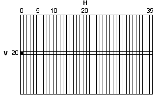 When the ball goes just beyond the right edge of the screen, it triggers an error because it exceeds the window limit of "39." Let's walk through each of the lines to discuss how each contributes to the final animated sequence and also to discuss some problems which exist in the program. Line 100 tells the computer to call up a fresh low-resolution graphics page. Line 1000 is simply a "remark" or "comment" line. Line 1040 sets a variable called H to zero and Line 1060 sets another variable called V to 20. The variable H will be used to define the position of the ball on the Horizontal axis and V will do the same on the Vertical axis. Note that since the ball will only be moving back and forth, the variable H will change, however V will not. Line 1080 chooses a color for the ball: two is the code for blue. Line 1100 finally plots a point at the screen location H,V which translates into a dot at the intersection of 0 across and 20 down. We have therefore completed the first stage of our "draw, erase, move, draw" animation model. The purpose of the next two lines is to erase the ball. Line 1120 chooses another color for drawing: zero is the code for black. Line 1140 again draws a ball at the same screen location H,V. However, since the ball is drawn in black the ball disappears because the background color of the screen is also black. Technically speaking, the ball was not erased, it was simply "painted over" in the same color as the background, so it vanishes. This little "trick" completes the second stage of our "draw, erase, move, draw" animation model. Line 1160 performs the mathematical calculation necessary to identify another screen location, in this case, the cell immediately to the right of the first. The command "LET H=H+1" loosely translates "make H what it was before plus 1." Since 0+1=1, H becomes 1. Mathematically incrementing the H variable simply tells the computer to "aim" at a different screen location which fulfills the third stage of our "draw, erase, move, draw" animation model. Line 1180 tells the computer to immediately branch to line 1080 and continue working from there. Line 1080 switches the drawing color back to blue. Line 1100 again plots a point at the screen location H,V. However, this time, H is now 1, so a blue ball is drawn at the intersection of 1 across and 20 down. This completes the first of many "draw, erase, move, draw" sequences necessary to move the ball across the screen. The program is now involved in a loop and will continue executing the loop until we tell it to stop (by pressing Control-C), the computer loses power, or something else unforeseen happens (like an error). Continuing the program's logic, line 1120 again changes the drawing color back to black. Line 1140 again draws a black ball over the blue ball which causes the ball to again disappear. Line 1160 again adds 1 to H, making it 2 and Line 1180 again branches the program back to 1080 starting the whole process over again. The program continues in the loop which causes it to continually draw, erase, move, and draw the ball over and over going from the left edge of the screen to the right. However, there are two major problems. One problem is perceptual and the other is technical. The technical problem is that this little program "crashes" upon reaching the right edge of the screen because there is no horizontal screen location at 40. The result is a rather rude and cryptic error message like "Illegal Quantity Error." However, this technical problem is easily dealt with, so we will deal with the perceptual problem first. When the program is actually run, the ball does not smoothly travel from left to right. Instead, it often appears as though it is "skipping" sporadically from left to right. The problem is not a computer malfunction, in fact, the computer is working too well. Even low-end microcomputer systems can process and execute this little program so fast that the blue ball is erased before the eye has time to actually perceive it. In order to give the eye a chance, we need to add a small delay to the program in the form of Lines 1110 and 1115:
Lines 1110 and 1115, in essence, give the computer "busy work" to perform, counting from 1 to 50 in this case, while the blue ball is displayed on the screen. This delays the program long enough at this crucial point to give the human eye a "long," clear view of the ball. These two lines will make a dramatic perceptual difference. The ball will now go smoothly from left to right when the program is run. However, remember that our goal was to have the ball bounce back and forth. So far, it travels only left to right. We also have to deal with the technical problem of the computer crashing when the ball goes over the right edge of the screen. The following changes take care of both issues:
The first thing you will probably notice is that the program is about twice as long as it was before. This is because it was copied and pasted below itself, starting with line 2000. These duplicated lines are identical to their counterparts from 1000-1180 with one simple, yet crucial exception. Line 2160, instead of adding 1 to H, subtracts 1. Adding makes the ball go from left to right, and subtracting makes the ball go from right to left (in other words, it "bounces"). Line 1170 and its counterpart at line 2170 were also added. These IF/THEN lines tell the computer to branch between the two parts of the program when the ball is about to go either too far to the right (i.e. H>39) or too far to the left (i.e. H<0). The result is a program which animates a little ball bouncing back and forth on the computer screen. |
GUI-Based Approaches to Fixed-Path Animation
The "draw, erase, move, draw" model also guides the development of fixed-path animation in GUI-based approaches. However, most GUI-based approaches do not use a mathematical model to produce fixed-path animation at the user interface level, even though mathematics may still underlie the animation sequence. Before discussing some examples of software designed expressly for the production of fixed-path animation, we will consider the simplest and oldest approach to animation -- frame-by-frame animation.
Frame-by-Frame Animation
Frame-by-frame animation, as the name implies, is when a set of successive frames is constructed so that when shown in rapid succession at just the right rate, one or more objects appear to move. This is the same technique that one would use to create paper and pencil animation where the object to be animated is drawn at slight variations from page to page. Animation is produced by flipping through the pages at just the right speed with your thumb. Frame-by-frame animation is the oldest form of animation and is the same technique used by the most sophisticated examples of film animation, such as Disney, whether drawn by hand or by computer. This is also the technique used in the labor-intensive "claymation" films, where real objects, such as bendable figurines, are moved slightly and photographed one frame at a time. (See Footnote 6)
Frame-by-frame animation requires that every detail between one frame and the next be exactly the same -- except for the object or objects being animated. These objects are drawn in small, but discrete, variations from the preceding frame. If the animation is shown at 30 frames per second, a standard video display rate, each frame shows the object in increments lasting one-thirtieth of a second. Reducing the animation to a rate of 10 frames per second, will, of course, be cheaper and quicker to produce, but the quality of the animation will suffer accordingly. Anyone who has seen and compared a classic Disney cartoon with typical Saturday morning television knows this quality difference firsthand. Even though the frames are discrete, the human perception system will fill in the gaps and perceive continuous movement (see chapter 4).
GUI computers make frame-by-frame animation readily available through their copy and paste features. In HyperCard on the Macintosh, for example, once the first frame, or card, is created, it can be copied and pasted as the second card, which, in turn, can be edited to change the appearance or position of the animated object. This and all succeeding frames can be copied, pasted, and revised as shown in Figure 3.17. When the entire sequence is shown at the proper rate, animation is produced.
Figure 3.18 shows a typical way some animation software packages accomplish frame-by-frame animation. In this particular case, the software allows for single objects to be animated "in place." Figure 3.18 shows a simple example to create the illusion of a spinning helicopter rotor. The software allows for any single frame to be created pixel by pixel and then copied over into the next frame for minute editing necessary to create the illusion. Animating a person running, a horse galloping, or clock hands revolving would be other examples of animation where this approach would be useful.
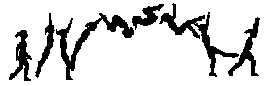
Figure 3.17
An example of frame-by-frame animation.
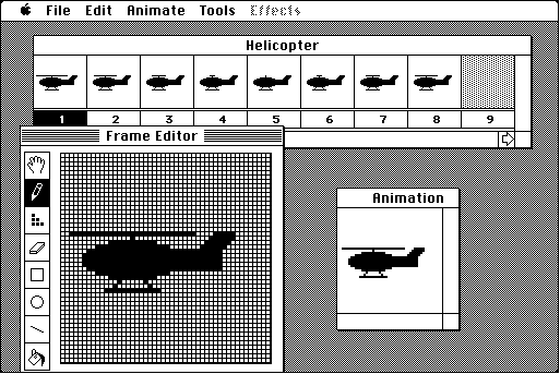
Figure 3.18
An example of a frame-by-frame animation package. When shown in rapid succession, the helicopter's blade will appear to spin.
Of course, it becomes a surprisingly complex task to keep track of even a few animated objects at a time. For this reason, some computer software packages separate the task of manipulating individual animated objects from the assembly of all the objects into one completed animation sequence. Several packages use the analogy of a movie production to do this. (See Footnote 7) Individual animated objects become the cast of characters. As shown in Figure 3.19, the entire animated production is called the "score" and consists horizontally of the individual frames and vertically of "tracks" on which cast members perform. Any one frame combines any number of animated objects, each on its own separate track. There are also separate tracks available for sound and special effects. When finished, the score can be rewound or fast-forwarded to any position and played, meaning that frames are then displayed one by one at a specified rate.
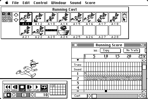
Figure 3.19
A snapshot of a sophisticated animation package that uses the analogy of a stage production.
Other GUI-Based Approaches to Producing Fixed-Path Animation
There are a variety of other ways to produce fixed-path animation. Some applications allow a user to move an object around the screen freehand while recording the motion in real-time. The software then automatically converts the information into frame-by-frame animation. Of course, if the user's hand shakes a little in the middle, it will be necessary to edit those particular frames. This is usually a more difficult task than first imagined. Other approaches allow for the path of the object to be defined first and edited, rather than the object itself.
The simplest methods for defining an animated path are those that animate an object along a straight line, as shown in Figure 3.20. The entire animated sequence is defined by the object to be animated, the two end points of the imaginary line along which the object moves, and the time (sometimes defined as speed) that the object takes to complete its "run." The object's initial screen position usually defines one end point. The object is then physically grabbed and moved to the other end point with the computer recording the time taken to get there. The sequence then can be fine-tuned until the desired effect is reached.
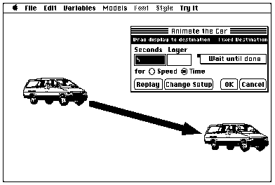
Figure 3.20
An example of "fixed destination" animation. All the user has to do is drag the object to be animated from the starting point to the ending point. The computer extrapolates all of the points in-between.
The next level of sophistication is animation along a crooked path, analogous to a piece of string. Again, the sequence has a starting point and an ending point. However, there are also one or more points along the way that "pull" on the string, as shown in Figure 3.21. Points can be added or deleted to the string. The points also can be defined to make the string go along a straight or curved line between the points.
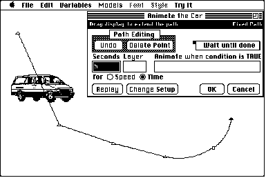
Figure 3.21
An example of fixed path animation. The animated path of the object can be continually extended and reshaped.
Data-Driven Animation
Command-based and GUI-based approaches to data-driven animation are quite similar. Each requires methods and techniques to keep track of one or more variables that control the animation of one or more screen objects. Even though many systems may capitalize on GUI features, all data-driven animation methods are essentially command-based approaches.
Recall the example of fixed-path animation using a command-based approach from Box 3.2. Rather than have the computer decide on the values of H and V, we can let them be determined by user interaction. We need some method of allowing the user to provide input to the computer system. For example, most computer keyboards have four arrow keys, one for each direction (i.e., left, right, up, and down). The computer can be programmed to move a screen object, such as the ball, in the direction of whatever arrow key is pressed or clicked on. Recall from our "bouncing ball" example that the variable H controlled horizontal motion and the variable V controlled vertical motion. The program can be easily modified to add 1 to H when the right arrow is pressed, or subtract 1 from H if the left arrow is pressed. Similarly, the program can add 1 to V when the down arrow is pressed and can subtract 1 from V when the up arrow is pressed. This simple program lets the user move, or drive, the ball anywhere on the screen.
With a little creativity, the program can be incorporated into a variety of instructional contexts: teaching how to follow map directions by adding a street background and having the user drive a car between points (as shown in Figure 3.22); or teaching latitude and longitude by switching to a nautical map and changing the object to a boat; having the object leave a trail, the program becomes an electronic Etch-A-Sketch; etc.
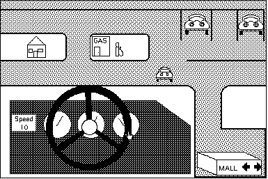
Figure 3.22
An example of data-driven animation. The user drives the car around the town just by pointing the hand icon on the steering wheel.
THE INSTRUCTIONAL DELIVERY OF COMPUTER GRAPHICS
Regardless of how static or animated graphics may be produced, the ultimate instructional question is how the computer graphics will be implemented or delivered in an instructional system. The most obvious delivery platform for computer graphics is the computer. This includes all instructional materials delivered by computer, such as computer-assisted instruction and computer-controlled presentations.
However, it is not always feasible to deliver the materials by computer, either because of economy or practicality. Probably the next most obvious delivery platform is print-based material. Computer animation presents unique concerns. Data-driven animation, by definition, must be delivered by computer because the student input must be processed moment to moment. Fixed-path animation, however, offers delivery alternatives. A practical solution to delivering fixed-path animation is to transfer the animation to videotape in order to take advantage of the widespread availability of videocassette players. However, several compromises must be made. Unless the user is willing to manually control the player, the program will be externally paced, an issue that must be included in the original design. Other problems are related to the quality of the video image, depending on the computer system used to produce the animation in the first place.
Computer systems and video systems vary widely in their methods of composing and transmitting a video signal. Video manufacturers typically use one of three signal systems to define the scan line: NTSC, PAL, and SECAM. NTSC, named after the American National Television Standards Committee that established it, is the most common in the United States. PAL, or Phase Alternation Line, is the system adopted throughout most of the United Kingdom, Europe, the Middle East, Africa, Australia, and South America. SECAM, short for séquential couleur á memoire, was developed in France. Computer manufacturers vary even more widely in the way images are transmitted, and few use a standard video signal. (See Footnote 8) Computer screens, as already mentioned, are based on the pixel, not the scan line. The lack of compatibility between computer and video displays poses problems when trying to transpose a signal from one platform to the other. It is usually necessary to use a special device to synchronize the computer and video signals, such as a "gen-lock" that locks the pulses generated on separate signals to a common beat. Standardization between computer and video displays is being recognized as a very real need, especially as computer- generated graphics are becoming more common in video productions (Parsloe, 1983).
REVIEW